Insights

Trading Options: Noise vs Signal

It’s no surprise to portfolio managers that gaps will emerge between a thesis on a trade and its actual performance. For proof, you can ask anybody who tried to short US duration in 2019 on the premise that the economy would not slip into recession. There’s still no recession, yet yields fell nearly 80 basis points.

For options traders, there’s an added degree of difficulty since options, unlike linear instruments, are exposed to path-dependency, which can be viewed as a highly technical term for luck. If a patch of high or low volatility hits, but not at the right time, then it could prove unprofitable.

As an example, let’s say an options trading firm (the “Firm”) has a high conviction that delivered volatility will be subdued for the next month so the Firm sells an at-the-money straddle to implement its view. Further, let’s assume the asset underlying the option trends away of the options strike prices and then quiets down until expiration. Even though the delivered volatility was quite low, the Firm’s trade may not have made any profit since the exposure of the options it sold is highly dependent on the proximity of the strike prices to the underlying price. In trading parlance, the Firm’s options “lost their greeks” [—or, in other words, changed in value as a result of sensitivities to the trends in the underlying asset—] before the delivered volatility of the underlying asset dropped.

The options market started to address path dependency concerns in the 1990s with the advent of variance and volatility swaps, or structured products that contractually payoff the difference between an agreed-upon implied and subsequent delivered volatility or variance. The beauty of these products is that they are designed to counter path dependency concerns. Unfortunately, they are almost always more expensive to trade than the more vanilla options. Thus, if you want to take views on volatility while also minimizing transaction costs, then you are left with good old-fashioned options, including their inherent path dependency risk.

Most professional option traders are well aware of how option exposures change, based on path dependency. Some will mitigate this risk by spreading out their option positions across various strike prices. But how many strikes can an options trader realistically trade and what is the proper framework to assess likely performance? In other words, what if options traders could account for path dependency without the need of a variance or volatility swap? Options traders potentially can do this by acknowledging that they might have hedged against the wrong implied volatility for the option they’re taking. By accounting for this, an options trader can actually more accurately pinpoint noises versus signals when evaluating trades or other variables.

To explain how, let’s start with a comparison of the predicted payoff and the actual payoff of owning a one-month 5% out-of-the-money put with an implied volatility of 18%.¹

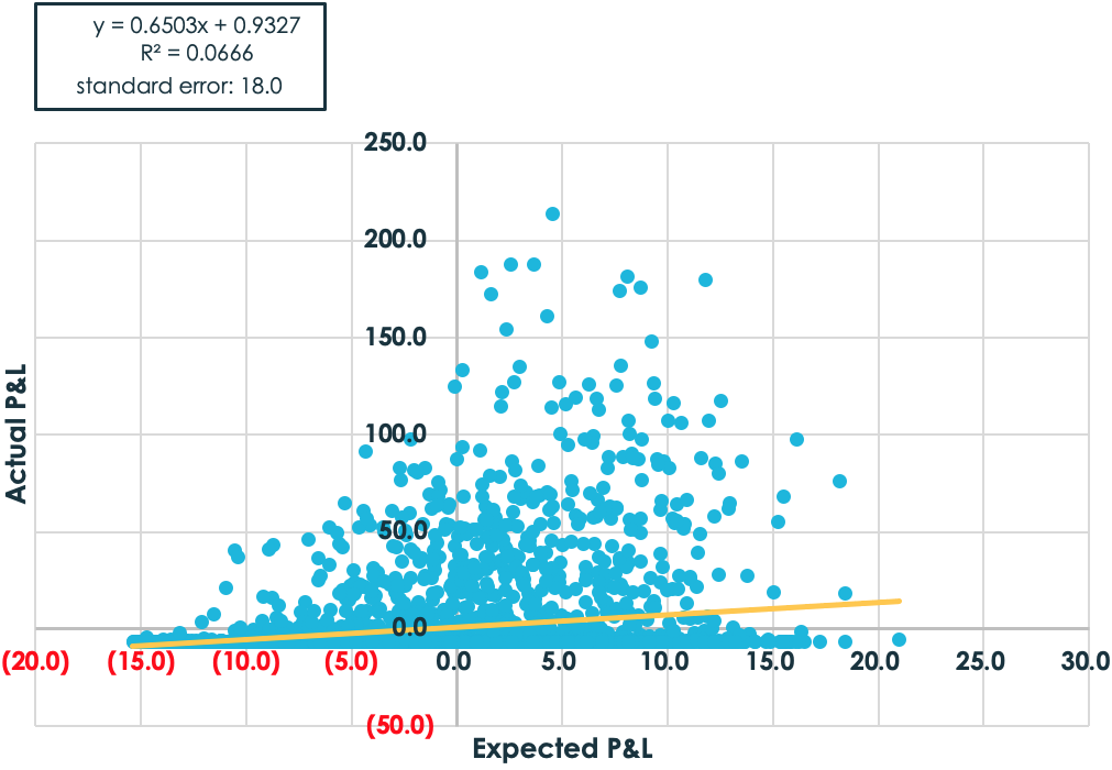
As the graph above suggests, the relationship between expected profitability and actual profitability is virtually non-existent. To be sure, as the expected profit and loss (P&L) rises, the actual gains are more likely to be positive. But the overall relationship is tenuous. Don’t forget this graph the next time someone suggests you should buy un-hedged puts because “volatility is cheap.”

Let’s see what happens when delta-hedging is included, which protects against price movements. Not surprisingly, a more predictable relationship between expected and actual performance starts to emerge.

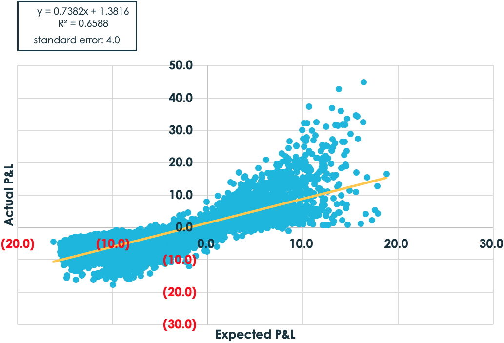
While there’s an improvement, a 4.0 volatility point standard of error isn’t necessarily reassuring when most volatility trades only have a few points of expected edge. To what degree, then, can the relationship be realistically improved even further?

The obvious choice for most option traders is to trade more than one strike. Here’s the graph based on trading strikes spaced 5% apart from 50% to 150% of the stock’s initial price.

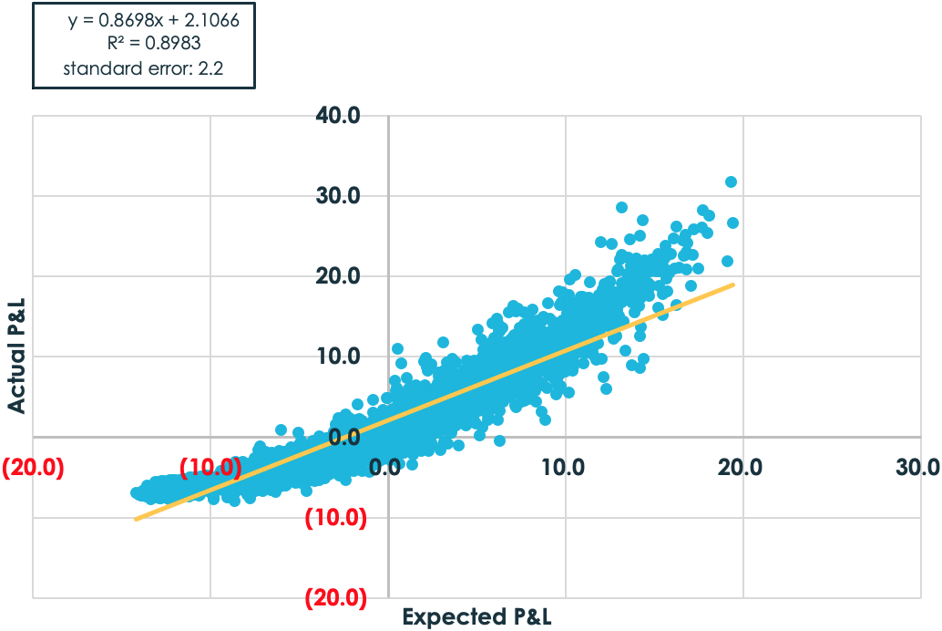
No shocker here. As the trader trades more strikes, its exposure to delta becomes more stable, thus making predictions easier. (On a side note, notice how the points start to form a curved relationship. This makes sense as option payoffs are convex but the expectation of P&L is linear.)

Of course, practically speaking, traders can’t always trade every strike, since some out-of-the-money strikes don’t exist or they have prohibitive transaction costs. Perhaps a more realistic assumption is that a trader can trade say, five, strikes from 90% moneyness to 110% moneyness, spaced 5% apart.

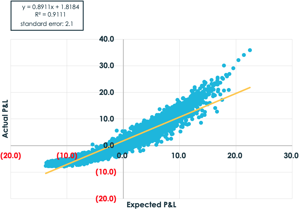
Now the result is a bit non-intuitive. There is a slight improvement in the relationship using fewer strikes. This is not what most traders would have assumed.

The reason for the improvement, despite fewer strikes? The act of delta-hedging options requires an assumption about the volatility for each option. Theory says that traders should hedge to the delivered volatility if they want to minimize variance of outcomes. Of course, the real world says good luck with finding a crystal ball that indicates what the delivered volatility will be at the time the trade was initiated. Sure, a trader can make an educated guess, but many option traders start with the assumption that the market is correct and then hedge to the implied volatilities. That’s critical because the option markets frequently impart what looks like a smile on implied volatility graphs. Within options, the smile shows the relationship between strike price and implied volatility. In equities, the smile is more of a skew, meaning that as strike prices decline, implied volatilities rise.

A practical implication of the skew is that if traders are going to hedge each option to its implied volatility, then they will implicitly hedge each option in their basket to a different volatility. That’s the cause of the apparent conundrum that more strikes hurt the prediction.

If you’re not convinced, then think about the many deep out-the-money puts that were bought in the above simulation with strike prices from 50% to 150% of the stock’s initial price. Those puts have a very high implied-volatility based on their strike price. As a result, and with the benefit of hindsight, the trader will have owned too much of the underlying, in most cases in, in his or her initial hedge.

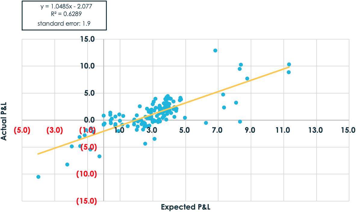
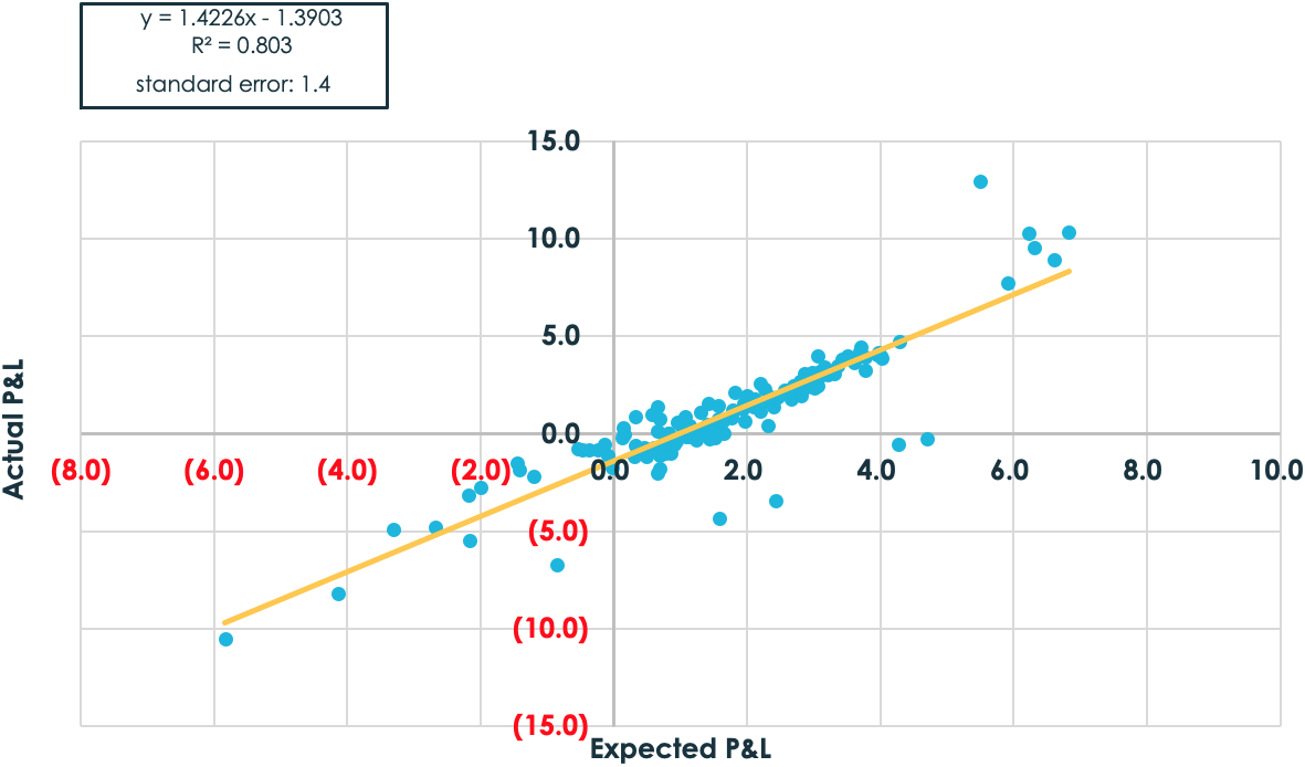
How then should these “hedging errors” be addressed? We suggest that traders incorporate them into their prediction of performance. Typically, traders would simply take the difference between delivered and implied volatility and multiply it by the volatility exposure. Instead, let’s add an additional term, which accounts for the fact that (in hindsight) the wrong volatility was used to hedge. While we’re at it, let’s also address the convexity issue as well. It’s easy to think linearly but traders really should adjust for the fact that options are non-linear instruments, as we explained. You can see how these two adjustments affected our predictions in the charts below.²

Both charts use the same five strikes that were traded before. Notice, however, the significant drop in the standard error in Method 2. By adjusting for convexity and, even more critical, accounting for the fact that the trades are hedged to the implied volatilities of each strike, the potential P&L outcomes are reduced and the results become much more linear.

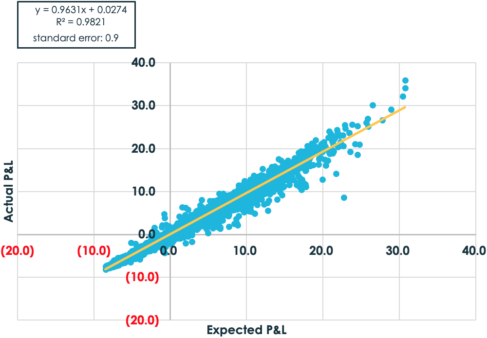
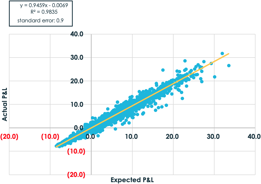
And here’s a comparison of the two methods using strikes spaced 5% apart from 50% to 150% moneyness. Notice the significant drop in standard error again.

Two questions remain. First, does this improved method of P&L estimation – and, therefore, a way to circumvent path dependency – actually work in the real world? Monte Carlo simulations were used in the previous charts, which are based on assumptions about the return distribution of stocks. The next charts do not. Instead, they are based on the results of a back-test of S&P 500 top-50 one-year dispersion trades from January 2008 to October 2019.

Notice the improvement in performance with the shift from the traditional method of thinking about volatility performance to the more nuanced approach.

Second, and more important, what should be done with this insight? To be sure, the enhanced method doesn’t predict either the direction or the volatility of the market. It does, however, provide a much better way to distinguish between the “noise” and the “signal” during the assessment of volatility trades, strategies or portfolio managers, without the need of that crystal ball.

Important Disclosures